10 minutes to Mars DataFrame
This is a short introduction to Mars DataFrame which is originated from 10 minutes to pandas.
Customarily, we import as follows:
In [1]: import mars

In [2]: import mars.tensor as mt

In [3]: import mars.dataframe as md
Now create a new default session.
In [4]: mars.new_session()
Out[4]: <mars.deploy.oscar.session.SyncSession at 0x7f8c65894050>
Object creation
Creating a Series by passing a list of values, letting it create
a default integer index:
In [5]: s = md.Series([1, 3, 5, mt.nan, 6, 8])

In [6]: s.execute()
Out[6]:
0    1.0
1    3.0
2    5.0
3    NaN
4    6.0
5    8.0
dtype: float64
Creating a DataFrame by passing a Mars tensor, with a datetime index
and labeled columns:
In [7]: dates = md.date_range('20130101', periods=6)

In [8]: dates.execute()
Out[8]:
DatetimeIndex(['2013-01-01', '2013-01-02', '2013-01-03', '2013-01-04',
               '2013-01-05', '2013-01-06'],
              dtype='datetime64[ns]', freq='D')

In [9]: df = md.DataFrame(mt.random.randn(6, 4), index=dates, columns=list('ABCD'))

In [10]: df.execute()
Out[10]:
                   A         B         C         D
2013-01-01 -1.365280  2.360637 -0.679526  0.358288
2013-01-02  2.557361 -0.078571  0.109942  0.191776
2013-01-03 -0.836771  0.123288  0.432302  1.342100
2013-01-04 -1.677534 -0.088742  0.708659 -0.161943
2013-01-05  1.620932 -0.686955  0.633519  0.907870
2013-01-06 -0.391767 -0.888535  0.867159 -2.279477
Creating a DataFrame by passing a dict of objects that can be converted to series-like.
In [11]: df2 = md.DataFrame({'A': 1.,
   ....:                     'B': md.Timestamp('20130102'),
   ....:                     'C': md.Series(1, index=list(range(4)), dtype='float32'),
   ....:                     'D': mt.array([3] * 4, dtype='int32'),
   ....:                     'E': 'foo'})
   ....:

In [12]: df2.execute()
Out[12]:
     A          B    C  D    E
0  1.0 2013-01-02  1.0  3  foo
1  1.0 2013-01-02  1.0  3  foo
2  1.0 2013-01-02  1.0  3  foo
3  1.0 2013-01-02  1.0  3  foo
The columns of the resulting DataFrame have different dtypes.
In [13]: df2.dtypes
Out[13]:
A           float64
B    datetime64[ns]
C           float32
D             int32
E            object
dtype: object
Viewing data
Here is how to view the top and bottom rows of the frame:
In [14]: df.head().execute()
Out[14]:
                   A         B         C         D
2013-01-01 -1.365280  2.360637 -0.679526  0.358288
2013-01-02  2.557361 -0.078571  0.109942  0.191776
2013-01-03 -0.836771  0.123288  0.432302  1.342100
2013-01-04 -1.677534 -0.088742  0.708659 -0.161943
2013-01-05  1.620932 -0.686955  0.633519  0.907870

In [15]: df.tail(3).execute()
Out[15]:
                   A         B         C         D
2013-01-04 -1.677534 -0.088742  0.708659 -0.161943
2013-01-05  1.620932 -0.686955  0.633519  0.907870
2013-01-06 -0.391767 -0.888535  0.867159 -2.279477
Display the index, columns:
In [16]: df.index.execute()
Out[16]:
DatetimeIndex(['2013-01-01', '2013-01-02', '2013-01-03', '2013-01-04',
               '2013-01-05', '2013-01-06'],
              dtype='datetime64[ns]', freq='D')

In [17]: df.columns.execute()
Out[17]: Index(['A', 'B', 'C', 'D'], dtype='object')
DataFrame.to_tensor() gives a Mars tensor representation of the underlying data.
Note that this can be an expensive operation when your DataFrame has
columns with different data types, which comes down to a fundamental difference
between DataFrame and tensor: tensors have one dtype for the entire tensor,
while DataFrames have one dtype per column. When you call
DataFrame.to_tensor(), Mars DataFrame will find the tensor dtype that can hold all
of the dtypes in the DataFrame. This may end up being object, which requires
casting every value to a Python object.
For df, our DataFrame of all floating-point values,
DataFrame.to_tensor() is fast and doesn’t require copying data.
In [18]: df.to_tensor().execute()
Out[18]:
array([[-1.36528022,  2.36063677, -0.67952625,  0.35828832],
       [ 2.55736127, -0.07857078,  0.10994215,  0.19177591],
       [-0.8367705 ,  0.12328824,  0.43230154,  1.34209999],
       [-1.6775344 , -0.08874234,  0.70865935, -0.16194346],
       [ 1.62093247, -0.68695487,  0.63351933,  0.90787014],
       [-0.39176732, -0.88853484,  0.86715906, -2.27947673]])
For df2, the DataFrame with multiple dtypes,
DataFrame.to_tensor() is relatively expensive.
In [19]: df2.to_tensor().execute()
Out[19]:
array([[1.0, Timestamp('2013-01-02 00:00:00'), 1.0, 3, 'foo'],
       [1.0, Timestamp('2013-01-02 00:00:00'), 1.0, 3, 'foo'],
       [1.0, Timestamp('2013-01-02 00:00:00'), 1.0, 3, 'foo'],
       [1.0, Timestamp('2013-01-02 00:00:00'), 1.0, 3, 'foo']],
      dtype=object)
Note
DataFrame.to_tensor() does not include the index or column
labels in the output.
describe() shows a quick statistic summary of your data:
In [20]: df.describe().execute()
Out[20]:
              A         B         C         D
count  6.000000  6.000000  6.000000  6.000000
mean  -0.015510  0.123520  0.345343  0.059769
std    1.714518  1.163762  0.565804  1.264232
min   -1.677534 -0.888535 -0.679526 -2.279477
25%   -1.233153 -0.537402  0.190532 -0.073514
50%   -0.614269 -0.083657  0.532910  0.275032
75%    1.117758  0.072823  0.689874  0.770475
max    2.557361  2.360637  0.867159  1.342100
Sorting by an axis:
In [21]: df.sort_index(axis=1, ascending=False).execute()
Out[21]:
                   D         C         B         A
2013-01-01  0.358288 -0.679526  2.360637 -1.365280
2013-01-02  0.191776  0.109942 -0.078571  2.557361
2013-01-03  1.342100  0.432302  0.123288 -0.836771
2013-01-04 -0.161943  0.708659 -0.088742 -1.677534
2013-01-05  0.907870  0.633519 -0.686955  1.620932
2013-01-06 -2.279477  0.867159 -0.888535 -0.391767
Sorting by values:
In [22]: df.sort_values(by='B').execute()
Out[22]:
                   A         B         C         D
2013-01-06 -0.391767 -0.888535  0.867159 -2.279477
2013-01-05  1.620932 -0.686955  0.633519  0.907870
2013-01-04 -1.677534 -0.088742  0.708659 -0.161943
2013-01-02  2.557361 -0.078571  0.109942  0.191776
2013-01-03 -0.836771  0.123288  0.432302  1.342100
2013-01-01 -1.365280  2.360637 -0.679526  0.358288
Selection
Note
While standard Python / Numpy expressions for selecting and setting are
intuitive and come in handy for interactive work, for production code, we
recommend the optimized DataFrame data access methods, .at, .iat,
.loc and .iloc.
Getting
Selecting a single column, which yields a Series,
equivalent to df.A:
In [23]: df['A'].execute()
Out[23]:
2013-01-01   -1.365280
2013-01-02    2.557361
2013-01-03   -0.836771
2013-01-04   -1.677534
2013-01-05    1.620932
2013-01-06   -0.391767
Freq: D, Name: A, dtype: float64
Selecting via [], which slices the rows.
In [24]: df[0:3].execute()
Out[24]:
                   A         B         C         D
2013-01-01 -1.365280  2.360637 -0.679526  0.358288
2013-01-02  2.557361 -0.078571  0.109942  0.191776
2013-01-03 -0.836771  0.123288  0.432302  1.342100

In [25]: df['20130102':'20130104'].execute()
Out[25]:
                   A         B         C         D
2013-01-02  2.557361 -0.078571  0.109942  0.191776
2013-01-03 -0.836771  0.123288  0.432302  1.342100
2013-01-04 -1.677534 -0.088742  0.708659 -0.161943
Selection by label
For getting a cross section using a label:
In [26]: df.loc['20130101'].execute()
Out[26]:
A   -1.365280
B    2.360637
C   -0.679526
D    0.358288
Name: 2013-01-01 00:00:00, dtype: float64
Selecting on a multi-axis by label:
In [27]: df.loc[:, ['A', 'B']].execute()
Out[27]:
                   A         B
2013-01-01 -1.365280  2.360637
2013-01-02  2.557361 -0.078571
2013-01-03 -0.836771  0.123288
2013-01-04 -1.677534 -0.088742
2013-01-05  1.620932 -0.686955
2013-01-06 -0.391767 -0.888535
Showing label slicing, both endpoints are included:
In [28]: df.loc['20130102':'20130104', ['A', 'B']].execute()
Out[28]:
                   A         B
2013-01-02  2.557361 -0.078571
2013-01-03 -0.836771  0.123288
2013-01-04 -1.677534 -0.088742
Reduction in the dimensions of the returned object:
In [29]: df.loc['20130102', ['A', 'B']].execute()
Out[29]:
A    2.557361
B   -0.078571
Name: 2013-01-02 00:00:00, dtype: float64
For getting a scalar value:
In [30]: df.loc['20130101', 'A'].execute()
Out[30]: -1.3652802178692118
For getting fast access to a scalar (equivalent to the prior method):
In [31]: df.at['20130101', 'A'].execute()
Out[31]: -1.3652802178692118
Selection by position
Select via the position of the passed integers:
In [32]: df.iloc[3].execute()
Out[32]:
A   -1.677534
B   -0.088742
C    0.708659
D   -0.161943
Name: 2013-01-04 00:00:00, dtype: float64
By integer slices, acting similar to numpy/python:
In [33]: df.iloc[3:5, 0:2].execute()
Out[33]:
                   A         B
2013-01-04 -1.677534 -0.088742
2013-01-05  1.620932 -0.686955
By lists of integer position locations, similar to the numpy/python style:
In [34]: df.iloc[[1, 2, 4], [0, 2]].execute()
Out[34]:
                   A         C
2013-01-02  2.557361  0.109942
2013-01-03 -0.836771  0.432302
2013-01-05  1.620932  0.633519
For slicing rows explicitly:
In [35]: df.iloc[1:3, :].execute()
Out[35]:
                   A         B         C         D
2013-01-02  2.557361 -0.078571  0.109942  0.191776
2013-01-03 -0.836771  0.123288  0.432302  1.342100
For slicing columns explicitly:
In [36]: df.iloc[:, 1:3].execute()
Out[36]:
                   B         C
2013-01-01  2.360637 -0.679526
2013-01-02 -0.078571  0.109942
2013-01-03  0.123288  0.432302
2013-01-04 -0.088742  0.708659
2013-01-05 -0.686955  0.633519
2013-01-06 -0.888535  0.867159
For getting a value explicitly:
In [37]: df.iloc[1, 1].execute()
Out[37]: -0.07857078157345845
For getting fast access to a scalar (equivalent to the prior method):
In [38]: df.iat[1, 1].execute()
Out[38]: -0.07857078157345845
Boolean indexing
Using a single column’s values to select data.
In [39]: df[df['A'] > 0].execute()
Out[39]:
                   A         B         C         D
2013-01-02  2.557361 -0.078571  0.109942  0.191776
2013-01-05  1.620932 -0.686955  0.633519  0.907870
Selecting values from a DataFrame where a boolean condition is met.
In [40]: df[df > 0].execute()
Out[40]:
                   A         B         C         D
2013-01-01       NaN  2.360637       NaN  0.358288
2013-01-02  2.557361       NaN  0.109942  0.191776
2013-01-03       NaN  0.123288  0.432302  1.342100
2013-01-04       NaN       NaN  0.708659       NaN
2013-01-05  1.620932       NaN  0.633519  0.907870
2013-01-06       NaN       NaN  0.867159       NaN
Operations
Stats
Operations in general exclude missing data.
Performing a descriptive statistic:
In [41]: df.mean().execute()
Out[41]:
A   -0.015510
B    0.123520
C    0.345343
D    0.059769
dtype: float64
Same operation on the other axis:
In [42]: df.mean(1).execute()
Out[42]:
2013-01-01    0.168530
2013-01-02    0.695127
2013-01-03    0.265230
2013-01-04   -0.304890
2013-01-05    0.618842
2013-01-06   -0.673155
Freq: D, dtype: float64
Operating with objects that have different dimensionality and need alignment. In addition, Mars DataFrame automatically broadcasts along the specified dimension.
In [43]: s = md.Series([1, 3, 5, mt.nan, 6, 8], index=dates).shift(2)

In [44]: s.execute()
Out[44]:
2013-01-01    NaN
2013-01-02    NaN
2013-01-03    1.0
2013-01-04    3.0
2013-01-05    5.0
2013-01-06    NaN
Freq: D, dtype: float64

In [45]: df.sub(s, axis='index').execute()
Out[45]:
                   A         B         C         D
2013-01-01       NaN       NaN       NaN       NaN
2013-01-02       NaN       NaN       NaN       NaN
2013-01-03 -1.836771 -0.876712 -0.567698  0.342100
2013-01-04 -4.677534 -3.088742 -2.291341 -3.161943
2013-01-05 -3.379068 -5.686955 -4.366481 -4.092130
2013-01-06       NaN       NaN       NaN       NaN
Apply
Applying functions to the data:
In [46]: df.apply(lambda x: x.max() - x.min()).execute()
Out[46]:
A    4.234896
B    3.249172
C    1.546685
D    3.621577
dtype: float64
String Methods
Series is equipped with a set of string processing methods in the str attribute that make it easy to operate on each element of the array, as in the code snippet below. Note that pattern-matching in str generally uses regular expressions by default (and in some cases always uses them). See more at Vectorized String Methods.
In [47]: s = md.Series(['A', 'B', 'C', 'Aaba', 'Baca', mt.nan, 'CABA', 'dog', 'cat'])

In [48]: s.str.lower().execute()
Out[48]:
0       a
1       b
2       c
3    aaba
4    baca
5     NaN
6    caba
7     dog
8     cat
dtype: object
Merge
Concat
Mars DataFrame provides various facilities for easily combining together Series and DataFrame objects with various kinds of set logic for the indexes and relational algebra functionality in the case of join / merge-type operations.
Concatenating DataFrame objects together with concat():
In [49]: df = md.DataFrame(mt.random.randn(10, 4))

In [50]: df.execute()
Out[50]:
          0         1         2         3
0  0.721489 -0.110345  0.735474 -1.641088
1  1.558771  0.756322 -1.118671 -0.281092
2  0.477267 -0.036496 -0.823793 -1.661408
3 -0.702555  0.048001 -1.102138  0.099206
4  0.941651  0.003015  1.207058 -1.889839
5 -0.764381 -1.811799  1.185082  0.045343
6 -1.456931  0.920873  2.029923 -1.988055
7 -1.190711 -1.122719 -0.108322 -2.085280
8  1.149432  0.433476  0.405015 -0.854277
9  0.103963 -0.977166 -1.684083 -1.272413

# break it into pieces
In [51]: pieces = [df[:3], df[3:7], df[7:]]

In [52]: md.concat(pieces).execute()
Out[52]:
          0         1         2         3
0  0.721489 -0.110345  0.735474 -1.641088
1  1.558771  0.756322 -1.118671 -0.281092
2  0.477267 -0.036496 -0.823793 -1.661408
3 -0.702555  0.048001 -1.102138  0.099206
4  0.941651  0.003015  1.207058 -1.889839
5 -0.764381 -1.811799  1.185082  0.045343
6 -1.456931  0.920873  2.029923 -1.988055
7 -1.190711 -1.122719 -0.108322 -2.085280
8  1.149432  0.433476  0.405015 -0.854277
9  0.103963 -0.977166 -1.684083 -1.272413
Join
SQL style merges. See the Database style joining section.
In [53]: left = md.DataFrame({'key': ['foo', 'foo'], 'lval': [1, 2]})

In [54]: right = md.DataFrame({'key': ['foo', 'foo'], 'rval': [4, 5]})

In [55]: left.execute()
Out[55]:
   key  lval
0  foo     1
1  foo     2

In [56]: right.execute()
Out[56]:
   key  rval
0  foo     4
1  foo     5

In [57]: md.merge(left, right, on='key').execute()
Out[57]:
   key  lval  rval
0  foo     1     4
1  foo     1     5
2  foo     2     4
3  foo     2     5
Another example that can be given is:
In [58]: left = md.DataFrame({'key': ['foo', 'bar'], 'lval': [1, 2]})

In [59]: right = md.DataFrame({'key': ['foo', 'bar'], 'rval': [4, 5]})

In [60]: left.execute()
Out[60]:
   key  lval
0  foo     1
1  bar     2

In [61]: right.execute()
Out[61]:
   key  rval
0  foo     4
1  bar     5

In [62]: md.merge(left, right, on='key').execute()
Out[62]:
   key  lval  rval
0  foo     1     4
1  bar     2     5
Grouping
By “group by” we are referring to a process involving one or more of the following steps:
Splitting the data into groups based on some criteria
Applying a function to each group independently
Combining the results into a data structure
In [63]: df = md.DataFrame({'A': ['foo', 'bar', 'foo', 'bar',
   ....:                          'foo', 'bar', 'foo', 'foo'],
   ....:                    'B': ['one', 'one', 'two', 'three',
   ....:                          'two', 'two', 'one', 'three'],
   ....:                    'C': mt.random.randn(8),
   ....:                    'D': mt.random.randn(8)})
   ....:

In [64]: df.execute()
Out[64]:
     A      B         C         D
0  foo    one -0.817412  1.310903
1  bar    one -1.909222 -0.886138
2  foo    two  0.048950  0.230002
3  bar  three  2.049341 -0.196978
4  foo    two  0.014524  0.932953
5  bar    two -1.052133 -0.033346
6  foo    one -0.859584 -0.332136
7  foo  three -1.174243 -1.556479
Grouping and then applying the sum() function to the resulting
groups.
In [65]: df.groupby('A').sum().execute()
Out[65]:
            C         D
A
bar -0.912014 -1.116463
foo -2.787764  0.585243
Grouping by multiple columns forms a hierarchical index, and again we can apply the sum function.
In [66]: df.groupby(['A', 'B']).sum().execute()
Out[66]:
                  C         D
A   B
bar one   -1.909222 -0.886138
    three  2.049341 -0.196978
    two   -1.052133 -0.033346
foo one   -1.676996  0.978767
    three -1.174243 -1.556479
    two    0.063474  1.162955
Plotting
We use the standard convention for referencing the matplotlib API:
In [67]: import matplotlib.pyplot as plt

In [68]: plt.close('all')
In [69]: ts = md.Series(mt.random.randn(1000),
   ....:                index=md.date_range('1/1/2000', periods=1000))
   ....:

In [70]: ts = ts.cumsum()

In [71]: ts.plot()
Out[71]: <AxesSubplot:>

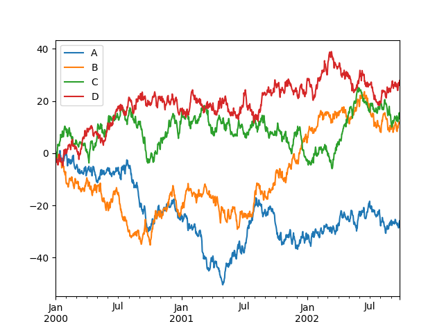
On a DataFrame, the plot() method is a convenience to plot all
of the columns with labels:
In [72]: df = md.DataFrame(mt.random.randn(1000, 4), index=ts.index,
   ....:                   columns=['A', 'B', 'C', 'D'])
   ....:

In [73]: df = df.cumsum()

In [74]: plt.figure()
Out[74]: <Figure size 640x480 with 0 Axes>

In [75]: df.plot()
Out[75]: <AxesSubplot:>

In [76]: plt.legend(loc='best')
Out[76]: <matplotlib.legend.Legend at 0x7f8c68104ed0>
Getting data in/out
CSV
In [77]: df.to_csv('foo.csv').execute()
Out[77]:
Empty DataFrame
Columns: []
Index: []
In [78]: md.read_csv('foo.csv').execute()
Out[78]:
     Unnamed: 0          A          B          C          D
0    2000-01-01  -0.119003  -0.192731   0.107914  -1.351706
1    2000-01-02  -0.895959   0.209087   0.446861  -1.760474
2    2000-01-03  -2.197316  -0.137080  -0.519755  -2.450023
3    2000-01-04  -1.697268   0.330867  -1.807150  -2.154578
4    2000-01-05  -1.938026  -0.522767  -1.235234  -2.716535
..          ...        ...        ...        ...        ...
995  2002-09-22 -27.504804  10.512483  13.645551  25.659550
996  2002-09-23 -28.630988  11.199417  13.026449  27.038196
997  2002-09-24 -27.836080  11.895768  14.176724  25.971726
998  2002-09-25 -26.394933  11.527917  15.501821  26.132438
999  2002-09-26 -25.899607  11.703820  14.459218  27.872741

[1000 rows x 5 columns]